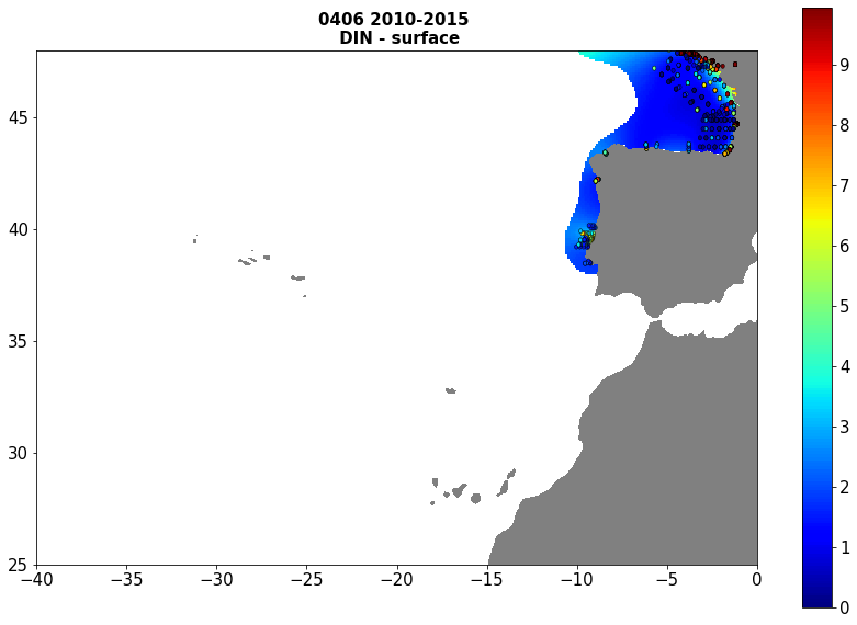
Moving 6-year analysis of Dissolved Inorganic Nitrogen at Atlantic Sea for each season. - winter: January-March, - spring: April-June, - summer: July-September, - autumn: October-December Every year of the time dimension corresponds to the 6-year centred average of each season. 6-year periods span - from 1988-1993 until 2015-2020 (winter), - from 1988-1993 until 2015-2020 (spring), - from 1986-1991 until 2015-2020 (summer), - from 1984-1989 until 2015-2020 (autumn). Observational data span from 1984 to 2020. Depth range (IODE standard depths): -2000.0, -1750, -1500.0, -1400.0, -1300.0, -1200.0, -1100.0, -1000.0, -900.0, -800.0, -700.0, -600.0, -500.0, -400.0, -300.0, -250.0, -200.0, -150.0, -125.0, -100.0, -75.0, -50.0,-40.0, -30.0, -20.0, -10.0, -5.0, -0.0 Data Sources: observational data from SeaDataNet/EMODNet Chemistry Data Network. Description of DIVA analysis: Geostatistical data analysis by DIVA (Data-Interpolating Variational Analysis) tool. GEBCO 1min topography is used for the contouring preparation. Analyzed filed masked using relative error threshold 0.3 and 0.5 DIVA settings. Correlation length was optimized and filtered vertically and a seasonally-averaged profile was used. Signal to noise ratio was fixed to 1. Logarithmic transformation applied to the data prior to the analysis. Background field: the data mean value is subtracted from the data. Detrending of data: no, Advection constraint applied: no. Units: umol/l

This visualization product displays the location of all the surveys present in the EMODnet marine litter database (MLDB). The different fishing gears used are represented by different colors. EMODnet Chemistry included the collection of marine litter in its 3rd phase. Since the beginning of 2018, data of seafloor litter collected by international fish-trawl surveys have been gathered and processed in the EMODnet Chemistry Marine Litter Database (MLDB). The harmonization of all the data has been the most challenging task considering the heterogeneity of the data sources, sampling protocols (OSPAR and MEDITS protocols) and reference lists used on a European scale. Moreover, within the same protocol, different gear types are deployed during fishing bottom trawl surveys. Unlike other EMODnet seafloor litter products, all trawls surveyed since 2006 are included in this map even if the wingspread and/or the distance are unknown. Only surveys with an unknown number of items were excluded from this product. More information on data processing and calculation are detailed in the document attached. Warning: the absence of data on the map doesn't necessarily mean that they don't exist, but that no information has been entered in the Marine Litter Database for this area.

This visualization product displays plastic bags density per trawl. EMODnet Chemistry included the collection of marine litter in its 3rd phase. Since the beginning of 2018, data of seafloor litter collected by international fish-trawl surveys have been gathered and processed in the EMODnet Chemistry Marine Litter Database (MLDB). The harmonization of all the data has been the most challenging task considering the heterogeneity of the data sources, sampling protocols (OSPAR and MEDITS protocols) and reference lists used on a European scale. Moreover, within the same protocol, different gear types are deployed during fishing bottom trawl surveys. In cases where the wingspread and/or number of items were unknown, data could not be used because these fields are needed to calculate the density. Data collected before 2011 are affected by this filter. When the distance reported in the data was null, it was calculated from: - the ground speed and the haul duration using this formula: Distance (km) = Haul duration (h) * Ground speed (km/h); - the trawl coordinates if the ground speed and the haul duration were not filled in. The swept area is calculated from the wingspread (which depends on the fishing gear type) and the distance trawled: Swept area (km²) = Distance (km) * Wingspread (km) Densities have been calculated on each trawl and year using the following computation: Density of plastic bags (number of items per km²) = ∑Number of plastic bags related items / Swept area (km²) Percentiles 50, 75, 95 & 99 have been calculated taking into account data for all years. Plastic bags reference codes taken into account for this product and information on data processing and calculation are detailed in the document attached p22. Warning: the absence of data on the map doesn't necessarily mean that they don't exist, but that no information has been entered in the Marine Litter Database for this area.

This visualization product displays fishing related items density per trawl. EMODnet Chemistry included the collection of marine litter in its 3rd phase. Since the beginning of 2018, data of seafloor litter collected by international fish-trawl surveys have been gathered and processed in the EMODnet Chemistry Marine Litter Database (MLDB). The harmonization of all the data has been the most challenging task considering the heterogeneity of the data sources, sampling protocols (OSPAR and MEDITS protocols) and reference lists used on a European scale. Moreover, within the same protocol, different gear types are deployed during fishing bottom trawl surveys. In cases where the wingspread and/or the number of items were unknown, data could not be used because these fields are needed to calculate the density. Data collected before 2011 are affected by this filter. When the distance reported in the data was null, it was calculated from: - the ground speed and the haul duration using this formula: Distance (km) = Haul duration (h) * Ground speed (km/h); - the trawl coordinates if the ground speed and the haul duration were not filled in. The swept area is calculated from the wingspread (which depends on the fishing gear type) and the distance trawled: Swept area (km²) = Distance (km) * Wingspread (km) Densities have been calculated on each trawl using the following computation: Density of fishing related items (number of items per km²) = ∑Number of fishing related items / Swept area (km²) Percentiles 50, 75, 95 & 99 have been calculated taking into account data for all years. Fishing related items reference codes taken into account for this product and information on data processing and calculation are detailed in the document attached p22. Warning: the absence of data on the map doesn't necessarily mean that they don't exist, but that no information has been entered in the Marine Litter Database for this area.

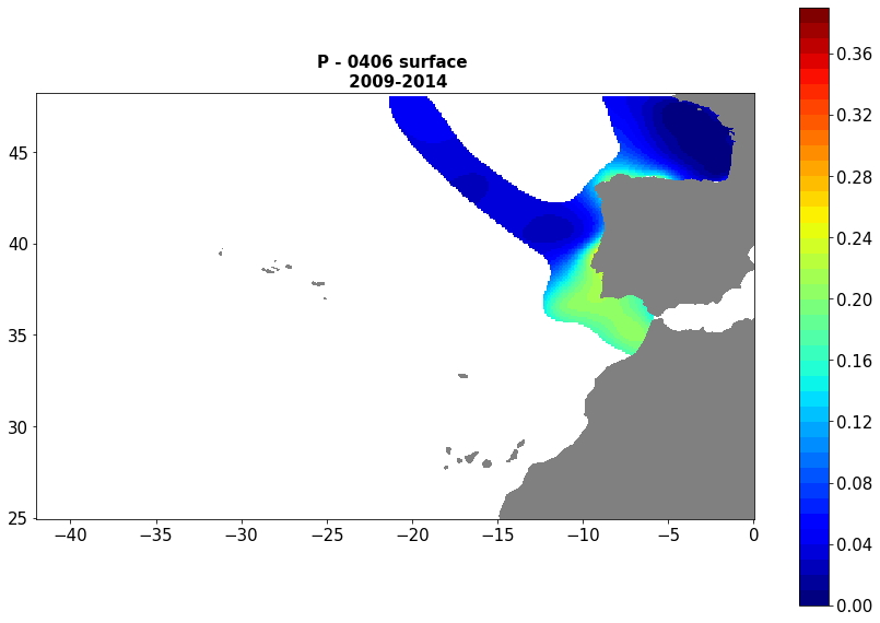
Moving 6-year analysis of Phosphate at Atlantic Sea for each season. - winter: January-March, - spring: April-June, - summer: July-September, - autumn: October-December Every year of the time dimension corresponds to the 6-year centred average of each season. 6-year periods span - from 1967-1972 until 2015-2020 (winter), - from 1960-1965 until 2015-2020 (spring), - from 1968-1973 until 2015-2020 (summer), - from 1961-1966 until 2015-2020 (autumn). Observational data span from 1960 to 2020. Depth range (IODE standard depths): -2000.0, -1750, -1500.0, -1400.0, -1300.0, -1200.0, -1100.0, -1000.0, -900.0, -800.0, -700.0, -600.0, -500.0, -400.0, -300.0, -250.0, -200.0, -150.0, -125.0, -100.0, -75.0, -50.0,-40.0, -30.0, -20.0, -10.0, -5.0, -0.0 Data Sources: observational data from SeaDataNet/EMODNet Chemistry Data Network. Description of DIVA analysis: Geostatistical data analysis by DIVA (Data-Interpolating Variational Analysis) tool. GEBCO 1min topography is used for the contouring preparation. Analyzed filed masked using relative error threshold 0.3 and 0.5 DIVA settings. Correlation length was optimized and filtered vertically and a seasonally-averaged profile was used. Signal to noise ratio was fixed to 1. Logarithmic transformation applied to the data prior to the analysis. Background field: the data mean value is subtracted from the data. Detrending of data: no, Advection constraint applied: no. Units: umol/l

Moving 6-year analysis of Silicate at Atlantic Sea for each season. - winter: January-March, - spring: April-June, - summer: July-September, - autumn: October-December Every year of the time dimension corresponds to the 6-year centred average of each season. 6-year periods span - from 1972-1977 until 2015-2020 (winter), - from 1984-1989 until 2015-2020 (spring), - from 1972-1977 until 2015-2020 (summer), - from 1971-1976 until 2015-2020 (autumn). Observational data span from 1971 to 2020. Depth range (IODE standard depths): -2000.0, -1750, -1500.0, -1400.0, -1300.0, -1200.0, -1100.0, -1000.0, -900.0, -800.0, -700.0, -600.0, -500.0, -400.0, -300.0, -250.0, -200.0, -150.0, -125.0, -100.0, -75.0, -50.0,-40.0, -30.0, -20.0, -10.0, -5.0, -0.0 Data Sources: observational data from SeaDataNet/EMODNet Chemistry Data Network. Description of DIVA analysis: Geostatistical data analysis by DIVA (Data-Interpolating Variational Analysis) tool. GEBCO 1min topography is used for the contouring preparation. Analyzed filed masked using relative error threshold 0.3 and 0.5 DIVA settings. Correlation length was optimized and filtered vertically and a seasonally-averaged profile was used. Signal to noise ratio was fixed to 1. Logarithmic transformation applied to the data prior to the analysis. Background field: the data mean value is subtracted from the data. Detrending of data: no, Advection constraint applied: no. Units: umol/l

Moving 6-year analysis and visualization of Water body dissolved inorganic nitrogen (DIN ) in the North Sea, four seasons: winter (dec-feb), spring (mar-may), summer (jun-aug), autumn (sep-nov). Data Sources: observational data from SeaDataNet/EMODnet Chemistry Data Network. Description of DIVA analysis: Geostatistical data analysis by DIVAnd (Data-Interpolating Variational Analysis) tool, version 2.7.2. results were subjected to the minfield option in DIVAnd to avoid negative/underestimated values in the interpolated results; error threshold masks L1 (0.3) and L2 (0.5) are included as well as the unmasked field. The depth dimension allows visualizing the gridded field at various depths.

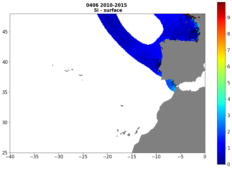
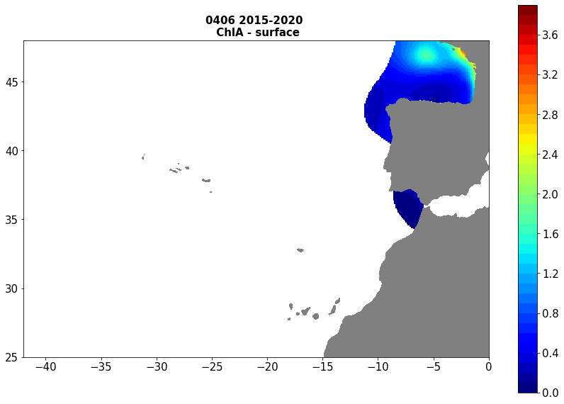
Moving 6-year analysis of Chlorophyll-a at Atlantic Sea for each season. - winter: January-March, - spring: April-June, - summer: July-September, - autumn: October-December Every year of the time dimension corresponds to the 6-year centred average of each season. 6-year periods span from 1972-1977 until 2012-2020. Observational data span from 1972 to 2020. Depth range (IODE standard depths): -300.0, -250.0, -200.0, -150.0, -125.0, -100.0, -75.0, -50.0,-40.0, -30.0, -20.0, -10.0, -5.0, -0.0 Data Sources: observational data from SeaDataNet/EMODNet Chemistry Data Network. Description of DIVA analysis: Geostatistical data analysis by DIVA (Data-Interpolating Variational Analysis) tool. GEBCO 1min topography is used for the contouring preparation. Analyzed filed masked using relative error threshold 0.3 and 0.5 DIVA settings. Correlation length was optimized and filtered vertically and a seasonally-averaged profile was used. Signal to noise ratio was fixed to 1. Logarithmic transformation applied to the data prior to the analysis. Background field: the data mean value is subtracted from the data. Detrending of data: no, Advection constraint applied: no. Units: mg/m^3

Moving 6-year analysis and visualization of Water body silicate in the North Sea, four seasons: winter (dec-feb), spring (mar-may), summer (jun-aug), autumn (sep-nov). Data Sources: observational data from SeaDataNet/EMODnet Chemistry Data Network. Description of DIVA analysis: Geostatistical data analysis by DIVAnd (Data-Interpolating Variational Analysis) tool, version 2.7.2. results were subjected to the minfield option in DIVAnd to avoid negative/underestimated values in the interpolated results; error threshold masks L1 (0.3) and L2 (0.5) are included as well as the unmasked field. The depth dimension allows visualizing the gridded field at various depths.

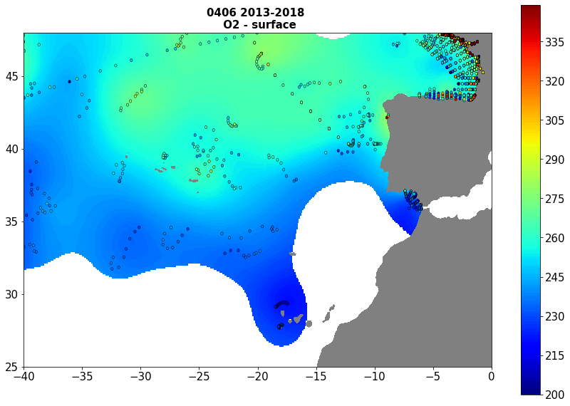
Moving 6-year analysis of Oxygen at Atlantic Sea for each season: - winter: January-March, - spring: April-June, - summer: July-September, - autumn: October-December. Every year of the time dimension corresponds to the 6-year centered average of each season. 6-year periods span from 1960-1965 until 2015-2020. Observational data span from 1960 to 2020. Depth range (IODE standard depths): -3000.0, -2500.0, -2000.0, -1750, -1500.0, -1400.0, -1300.0, -1200.0, -1100.0, -1000.0, -900.0, -800.0, -700.0, -600.0, -500.0, -400.0, -300.0, -250.0, -200.0, -150.0, -125.0, -100.0, -75.0, -50.0,-40.0, -30.0, -20.0, -10.0, -5.0, -0.0 Data Sources: observational data from SeaDataNet/EMODNet Chemistry Data Network. Description of DIVA analysis: Geostatistical data analysis by DIVA (Data-Interpolating Variational Analysis) tool. GEBCO 1min topography is used for the contouring preparation. Analyzed filed masked using relative error threshold 0.3 and 0.5 DIVA settings. Correlation length was optimized and filtered vertically and a seasonally-averaged profile was used. Signal to noise ratio was fixed to 1. Background field: the data mean value is subtracted from the data. Detrending of data: no, Advection constraint applied: no. Units: umol/l