 Metadata catalogue
Physical oceanography
Type of resources
Available actions
Topics
INSPIRE themes
Keywords
Contact for the resource
Provided by
Years
Formats
Update frequencies
Resolution
-
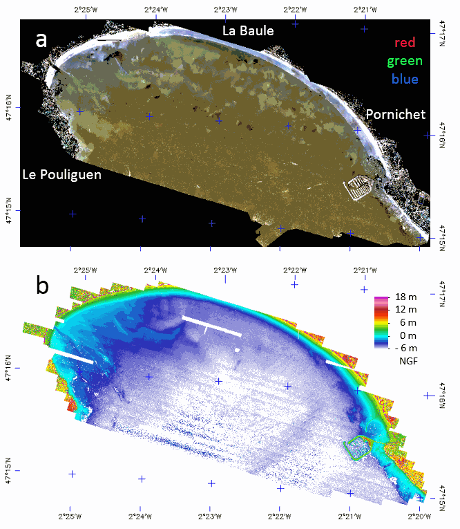
The LiDAR used is the Titan DW 600 from Teledyne Optech of the “Platform topo-bathymétrique aéroportée Nantes-Rennes”. Both 532-nm and 1064-nm LiDAR swath were acquired 6th and 7th of October 2017, at 400 m above ground with a FOV of 28° giving strip image width of 199.5 m with a nominal footprint of 0.49 m along-track and 0.29 m cross-track. A mirror compensation and a sidelap of 30% was used to prevent empty space between strips. The effective incident angle range was from 4 to 20°. The aircraft speed being 201.7 km/h the down track footprint rise up to 0.98 m on sideway what justify a final spatial resolution of 1 m. The laser pulse frequency was set to 50 kHz (100 kHz locally) giving an overall mean point density of 3.52 points/m². The full-waveform (FWF) was recorded only in 532-nm with a maximum length of 60 m, at 1 GHz frequency, resulting in a vertical resolution of 0.15 m. The Optech LiDAR Mapping Suite (LMS) combines a Global Positioning System (GPS) and Inertial Measurement Unit (IMU) to provide a georeferenced point cloud and associated FWF with strip optimization. To compute the complete point cloud, LMS uses an analogous approach to photogrammetric block adjustment. On overlap areas between each flight line, planes (typically roofs in land) are extracted and used in a least squares adjustment model provided by LMS. The trajectory accuracy provided by GEOFIT Company was better than 0.15 m in planimetry and 0.08 m on elevation. The set of data is stored in a zip file composed of the following image files associated with ENVI headers which are text files describing the image format. - LaBaule_2017106-7-orthophoto: contain the mosaic of RGB image acquired with the camera associated to the LiDAR. - LaBaule_2017106-7_536nm_raytracing-incident_angles_2m: contains the effective incident angle of each pixel retained in the mosaic with a pixel FOV of 0.3° and with a tilling of image strips in the top of each other from the North to the South. - LaBaule_2017106-7_1064nm_raytracing_discrete_echo_ranges_2m: contains the elevation of the water surface of each pixel. - LaBaule_2017106-7_536nm_raytracing_FWF_2m: contains the row FWF projected on the image plane at 0 m NGF with an offset of 30 m for easy spectral processing of the FWF (true range are stored in band names). - LaBaule_2017106-7_536nm_raytracing_FWF_2m_intensity_stats: contains the basic statistics of the FWF intensities. - LaBaule_2017106-7_536nm_raytracing_FWF_2m_range_stats: contains the min, max and thickness of the FWF ranges. - LaBaule_2017106-7_536nm_raytracing_FWF_2m_row_results: contains the row results of water surface and method 1 (dddNCFWF echoes) and method 2 (NCFWFT-1 bottoms) bathymetries as defined in https://doi.org/10.3390/rs11020117. - LaBaule_2017106-7_536nm_raytracing_FWF_4m_final_bathymetry: contains the final (cleaned NCFWFT-1 bottoms) bathymetry. The same data were acquired the 11th of August 2018 during a low tide with the same settings without RGB camera but with a new FWF recorder giving a lot less noisy signal allowing a constant spatial resolution of 1 m. The set of data is stored in a zip file composed of the following image files associated with ENVI headers which are text files describing the image format. - LaBaule_20180811_536nm_raytracing-incident_angles_1m: contains now 3 channels for the effective incident angle, the strip number and the GPS time. - LaBaule_20180811_1064nm_raytracing_discrete_echo_ranges_1m: contains the elevation of the water surface and all echoes above it in each pixel. - LaBaule_20180811_536nm_raytracing_FWF_1m: contains the row FWF projected on the image plane at 0 m NGF with an offset of 30 m for easy spectral processing of the FWF (true range are stored in band names). - LaBaule_20180811_536nm_raytracing_FWF_1m_intensity_stats: contains the basic statistics of the FWF intensities. - LaBaule_20180811_536nm_raytracing_FWF_1m_range_stats: contains the min, max and thickness of the FWF ranges. - LaBaule_20180811_536nm_raytracing_FWF_1m_row_results: contains the row results of water surface and method 1 (dddNCFWF echoes) and method 2 (NCFWFT-1 bottoms) bathymetries as defined in https://doi.org/10.3390/rs11020117. - LaBaule_20180811_536nm_raytracing_FWF_1m_final_bathymetry: contains the best of dddNCFWF echoes and NCFWFT-1 bottoms simply presented with the application of a 5x5 median filter. -
-
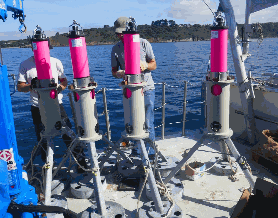
In the framework of the ERC FOCUS project, the Geosciences Ocean Laboratory (LGO) organized, from July 22 to 26, 2019, an experiment of seafloor geodesy in the Bay of Brest, entitled Geodesea-2019. The aim was to test acoustic beacons acquired for the FOCUS project and to test experimental protocols for seafloor positioning. The experiment was carried out from the Albert Lucas research station-vessel. The experiment was conducted in collaboration with the Laboratoire Environnement et Sociétés (LIENSs) from la Rochelle and the iXBlue company, in Brest. Relative acoustic ranging was carried out during four days, each beacon ranging the other ones at a regular time interval, while acquiring auxiliary data (temperature, pressure, sound-speed) to be able to convert travel-times into distances. Absolute positioning of the beacons on the seafloor was also carried out using a small Unmanned Surface Vehicle (USV) on which a compact GNSS/Acoustic system was mounted, combining an Ultra Short Baseline (USBL), an inertial system (INS) and a GNSS receiver.
-
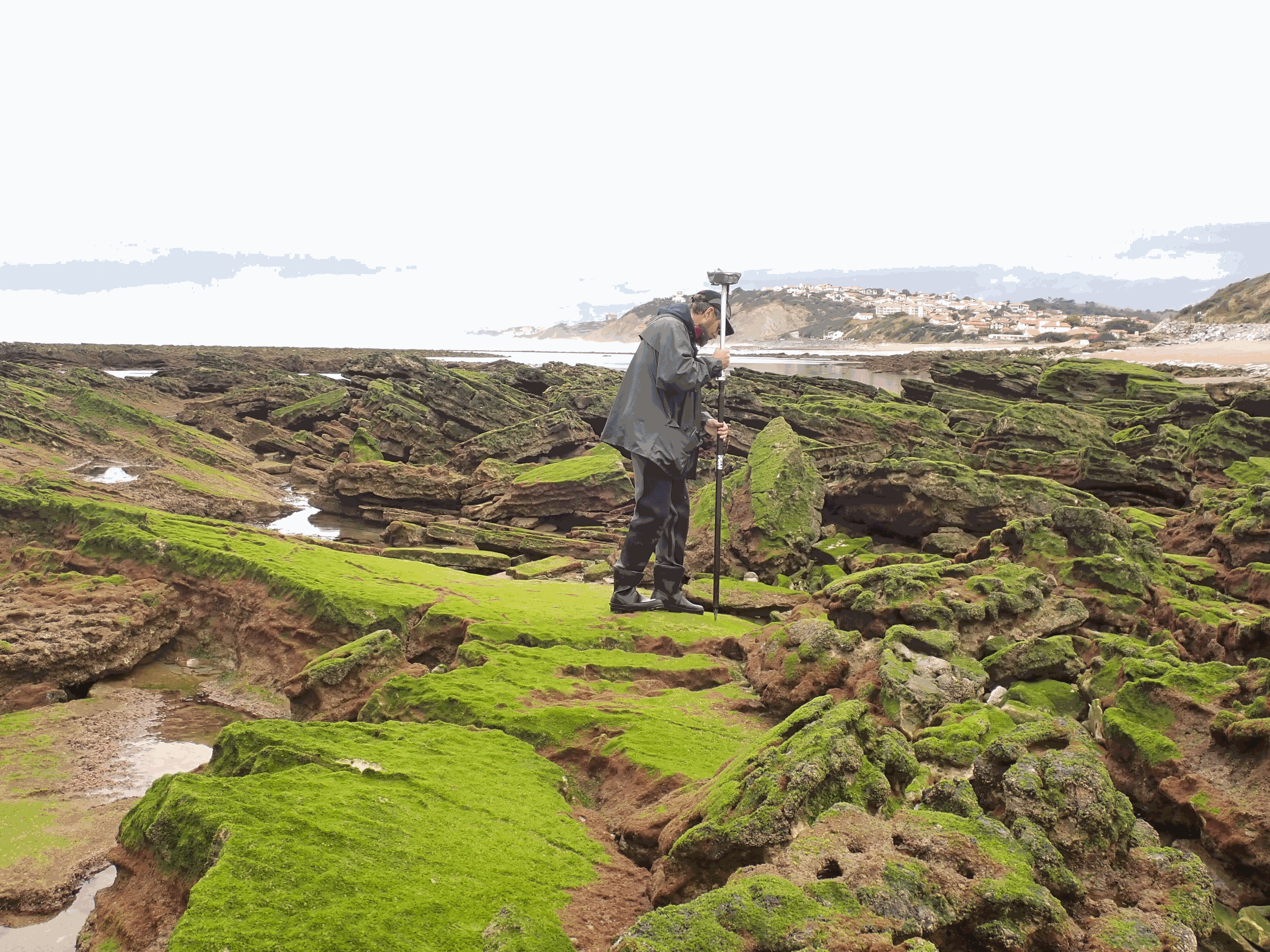
The present dataset is based on a nine site study of fine seabed topography in intertidal zones. Four coral sites (Maupiti A, B and C and Niau islands) and five rocky sites (Ars en Ré, Socoa, Parlementia A and B and Banneg island) have been explored. The data has been gathered using on-foot GNSS RTK for all sites (Trimble R8/R8S and Leica sytems) except Banneg island, where aerial Lidar data from Litto3D program has been used. The horizontal resolution varies between 3.8 and 12cm allowing to describe a wide range of spatial scales (generally over 3 spectral decades). The data has been processed to explore the statistical and spectral metrics which can be used to characterize the architectural complexity of seabeds.
-
A 30-year (1971-2000) temperature and salinity climatology is presented for surface and near-bed regions of the NW European shelf seas, with a resolution of 1/6 longitude by 1/10 latitude. The data have been extracted from the International Council for the Exploration of the Sea (ICES) data centre and supplemented by additional records from the World Ocean Data Centre (WODC). From the original data, which are irregularly distributed in space and time, the mean monthly temperature and salinity are calculated, as well as the climatic mean annual cycle. The climatology presented here is an improvement upon all existing climatologies presented in the literature for the NW European shelf; covering a wider area on a finer scale and including the surface and near-bed distribution of both temperature and salinity. Comparison of our data with existing climatologies shows good agreement, with differences occurring where our climatology is an improvement. This climatology, which will prove to be valuable to many users in the marine community will be regularly updated and made available to all users via the ICES data centre.
-
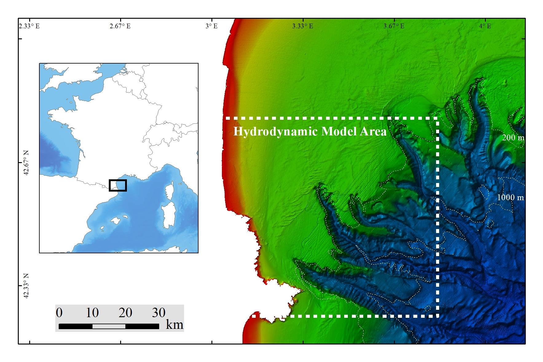
Extreme percentiles (1%, 5%, 95%, 99%) of bottom temperature and salinity, as well as (95%, 99%) of bottom currents, were modeled using SYMPHONIE on a numerical domain covering 65 × 60 km at a resolution of 80 m. The 10-m bathymetry used inside the Lacaze-Duthiers Canyon was collected during the CALADU_2021 cruise (https://doi.org/10.17600/18001575). Statistics of extreme values were derived from hourly fields simulated between November 1, 2012, and April 15, 2014. This period includes two contrasting winters: the winter of 2012–2013, which was cold with dense water cascading, and the winter of 2013–2014, which was warm. This dataset was produced to assess the probable distribution of habitats (habitat suitability modeling) for cold-water corals in the Lacaze-Duthiers Canyon at different resolutions as part of the European H2020 project REDRESS (Restoration of Deep-Sea Habitats to Rebuild European Seas, https://redress-project.eu/, Grant Agreement No. 101135492). SYMPHONIE is a component of the national service SIROCCO (research infrastructure ILICO). This dataset is related to the article "Mapping and Conservation of Cold-Water Corals in the Lacaze-Duthiers Canyon for Transboundary Management", submitted to Mediterranean Marine Science by Fabri et al. in 2025.
-

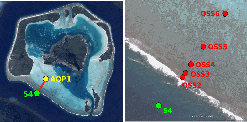
Bathymetric data were acquired in Reao Atoll, a semi-enclosed atoll lagoon without reef pass but connected to ocean through numerous shallow spillways (known locally as "hoa") along its southern rim. This data was acquired as part of the GAIA (ManaGement strAtegy evaluatIon for small-scale fisheries in Atoll lagoons) project, which evaluates the sustainability of giant clam exploitation within the context of climate change. The lagoon of Reao is composed of three basins with varying depths (the NW basin being the shallowest and the SE basin the deepest). Bathymetric data were acquired from 29/04/2022 to 04/05/2022, within the lagoon with a Multibeam echo sounder IWBMS (NORBIT), and resampled at 5 m spatial resolution. Satellite-derived-bathymetry (SDB) at 10 m spatial resolution was established by coupling this bathymetric data with a Sentinel-2B image captured on 26/09/2020 and using the « Iterative Multi Band Ratio » technique (detailed methodology is described in Quéré et al. 2025). Finally, bathymetric surveys were carried out to characterize the nine most functional hoa of the atoll. One bathymetric survey was carried out in the longitudinal section of each hoa, while one or two surveys were carried out in their cross-sections.
-
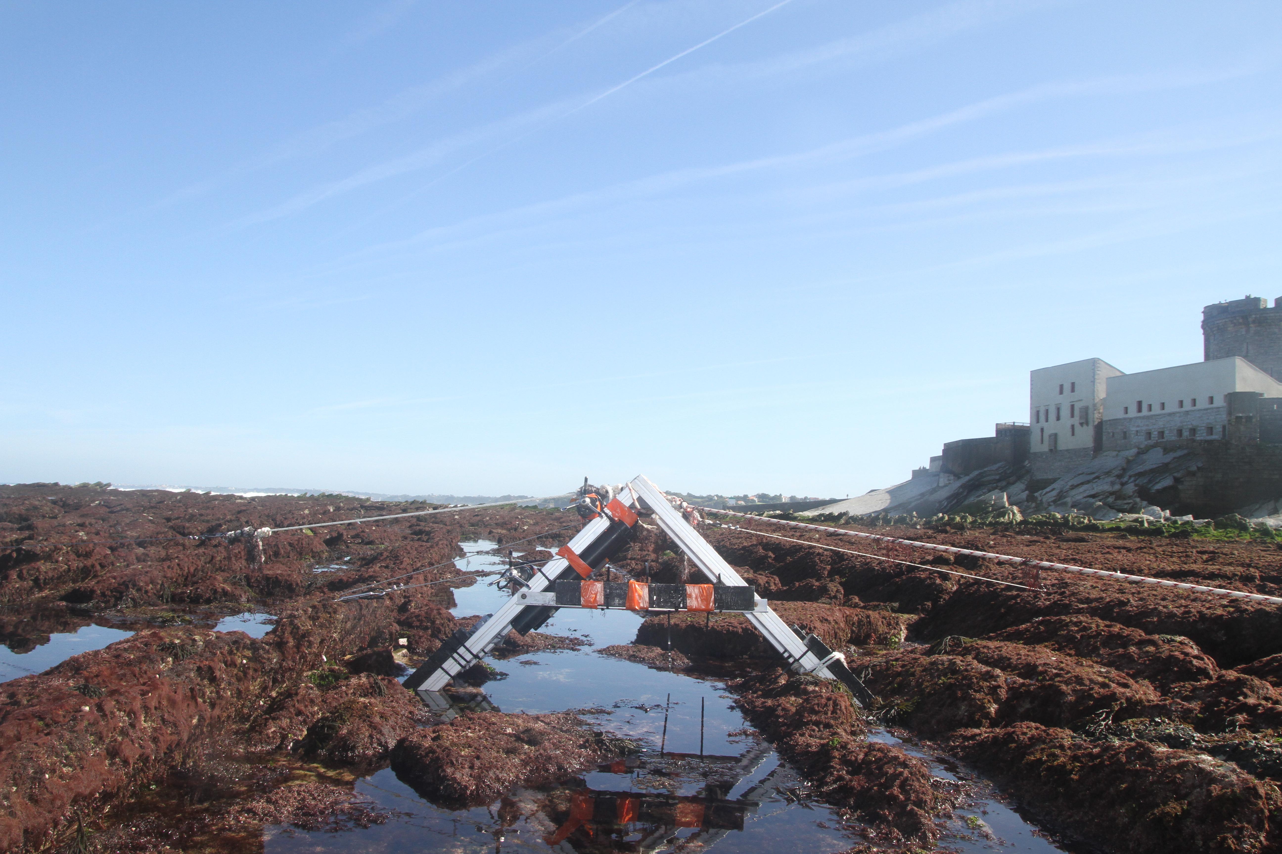
The database displays the field measurements recover during a one-week experiment in October 2021 on the Socoa's rocky platform, France. The general objective of the study was to evaluate the momentum balance over the rocky platform, in particular to quantifiy the combined effect of high seabed roughness and waves on the coupling between circulation, wave force and mean water level. The analysis is performed along a single cross-shore transect. The data include: - the cross-shore bathymetric profile - the time-series of integrated wave parameters, local mean water depth and wave-averaged currents over successive 30-min bursts - the depth- and wave-averaged momentum fluxes following the formulation proposed by Smith 2006 and Bruneau et al. 2011. The fluxes are median values obtained over significant wave height to depth ratio bins
-

The Gambier lagoon has a diamond-shaped form and surrounds seven high islands that are very exposed to the ocean. It is bordered by a barrier reef, which is submerged along the southern and western sides and by an intertidal to emerged barrier reef along the northern and eastern sides. The northern side is cut in some sections by several hoa, (shallow passages) allowing connections between the lagoon and the open ocean. The average depth of the domain is 25 m, with a maximum depth of 80 m along the southeastern coast of Mangareva Island. The bathymetry is complex, forming several basins, including the Rikitea enclosed lagoon, which is bordered by Mangareva and Aukena islands. The bathymetry of the Gambier Islands lagoon was generated using three data sources: SHOM soundings acquired in the 1960s, multi-beam data from Geopolynesie (5 m resolution) collected between 2020 and 2021, and satellite-derived bathymetry (SDB) at 10 m resolution using Sentinel-2 imagery to fill depth gaps in shallow areas. The final bathymetric grid was produced for implementation in the numerical hydrodynamic model MARS3D at a resolution of 100 m, using the compiled sounding datasets described above. The interpolation process included a Hanning low-pass filter applied five consecutive times for depths below 50 m, followed by an additional low-pass filter (ROMS) with a factor of 0.25.
-
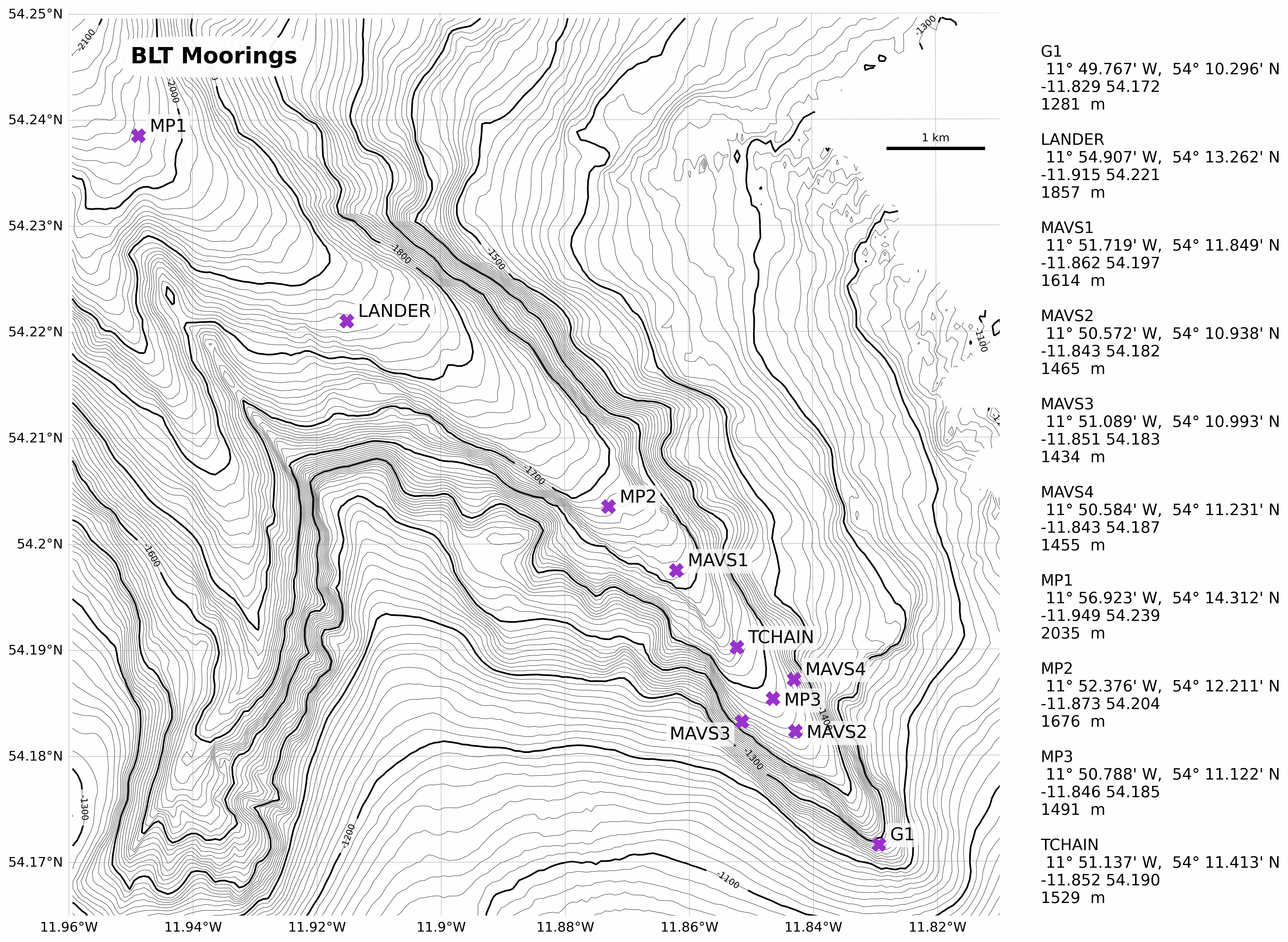
These data were collected as part of the Boundary Layer Turbulence and Abyssal Recipes (BLT Recipes) Experiment which focused on near-bottom processes within a continental slope canyon on the eastern side of the Rockall Trough, off Ireland. This specific dataset contains a bathymetry product based on data collected with the shipboard multibeam on RRS Discovery during cruises in 2021 and 2022.
-
Maupiti ("the Stuck Twins'') is a diamond-shaped island located in the western part of the Society archipelago in French Polynesia. The present study focuses on the data recovered over a single cross-barrier transect located in the south-west barrier during the MAUPITI HOE field campaign, from 5 to 18 July 2018. The studied area is representative of the reef structure observed along the 4km-long southwestern barrier reef, showing an alongshore-uniform structure exposed to swell approaching with weak incident angles, a healthy reef colony. In the cross-barrier direction, the reef displays a clear partitioning of bottom roughness that ranges from low-crested compact structures at the reef crest to higher and sparser coral bommies on the backreef. The experimental setup was specifically designed to analyse and differentiate the dynamics over three roughness-contrasting sections found over the barrier reef.