In order to demonstrate the density of accommodation along the Irish Coast all accommodation points provided by Failte Ireland where processed by using kernel density analysis to aggregate points which are spatially clustered, highlighting areas of high density. Data points were plotted from a Fáilte Ireland Accommodation dataset. Using Kernel Density, a raster of high to low density was produced and contours demonstrating the transitions were created. These polylines were then merged with the bounds of a 25km buffer polygon to create a polygon. The separate polygons were then categorised into their different categories similar to the original raster.

This Illustrates the existence or planned presence of marine renewable energy sites (wind farm authorisations) in Irish waters, as catalogued and displayed by 4C Offshore and DP Energy. The features were digitized manually from visualisations of windfarm authorisations viewable on https://www.4coffshore.com/offshorewind/ while the location for Inis Ealga was supplied in a shapefile provided by DP Energy. The research was undertaken by the MaREI Centre for Marine and Renewable Energy and published in 2019.

The location of seabed gas pipeline infrastructure from Cork to the Kinsale platform, Mayo to the Corrib platform and the international connector routes between Ireland and Scotland.

The National Marine Planning Framework (NMPF) Area is the geographic area management and reporting unit for Ireland's NMPF reporting. The NMPF sits at the top of the hierarchy of plans and sectoral policies for the marine area of Ireland. Marine planning brings together multiple users of the ocean to make informed and coordinated decisions on the sustainable use of marine resources. EU Directive 2014/89/EU, establishing a framework for maritime spatial planning, was adopted in July 2014. The European Union (Framework for Maritime Spatial Planning) Regulations 2016 were signed into law on 29th June 2016. The NMPF is managed by the Department of Housing Planning and Local Government (DHPLG) with monitoring support provided by the Marine Institute. The area applies from the High Water Mark in Ireland’s coastal waters, territorial seas, exclusive economic zone and in designated parts of the continental shelf. Ireland’s marine area totals over 488,000 Km2.

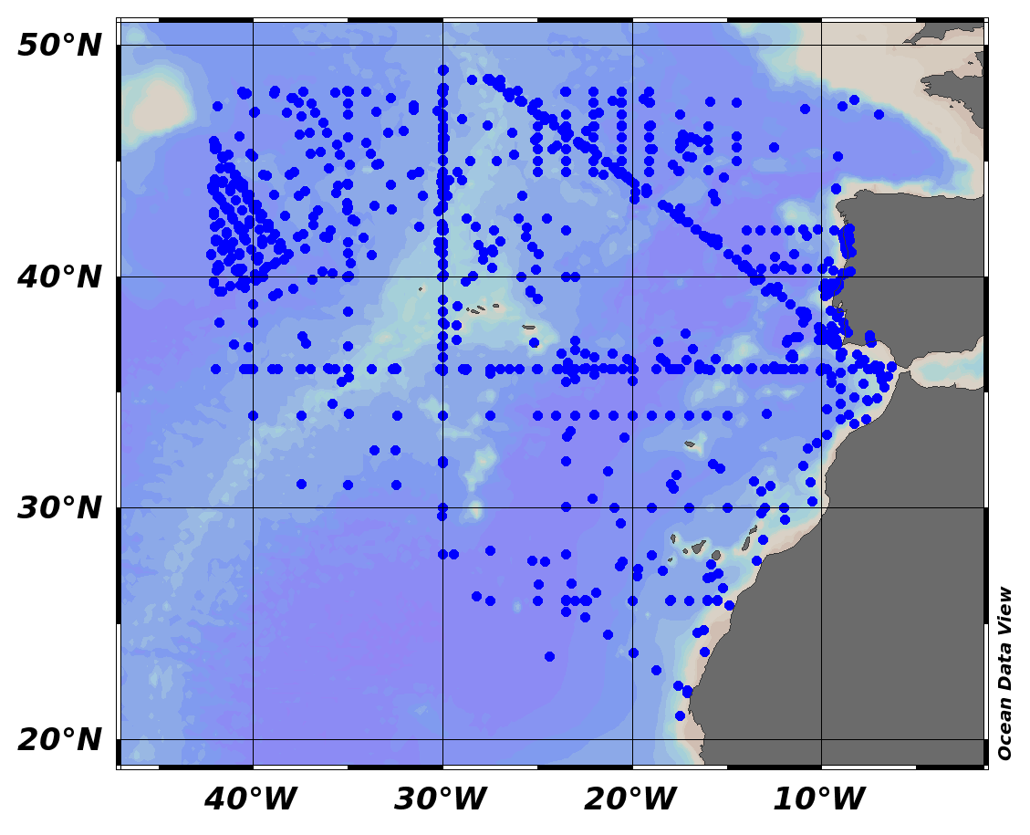
EMODnet Vessel Density Map were created by Cogea in 2019 in the framework of EMODnet Human Activities, an initiative funded by the EU Commission. The maps are based on AIS data purchased by CLS and show shipping density in 1km*1km cells of a grid covering all EU waters (and some neighbouring areas). Density is expressed as hours per square kilometre per month. A set of AIS data had to be purchased from CLS, a commercial provider. The data consists of messages sent by automatic tracking system installed on board ships and received by terrestrial and satellite receivers alike. The dataset covers the whole 2017 for an area covering all EU waters. A partial pre-processing of the data was carried out by CLS: (i) The only AIS messages delivered were the ones relevant for assessing shipping activities (AIS messages 1, 2, 3, 18 and 19). (ii) The AIS DATA were down-sampled to 3 minutes (iii) Duplicate signals were removed. (iv) Wrong MMSI signals were removed. (v) Special characters and diacritics were removed. (vi) Signals with erroneous speed over ground (SOG) were removed (negative values or more than 80 knots). (vii) Signals with erroneous course over ground (COG) were removed (negative values or more than 360 degrees). (viii) A Kalman filter was applied to remove satellite noise. The Kalman filter was based on a correlated random walk fine-tuned for ship behaviour. The consistency of a new observation with the modeled position is checked compared to key performance indicators such as innovation, likelihood and speed. (ix) A footprint filter was applied to check for satellite AIS data consistency. All positions which were not compliant with the ship-satellite co-visibility were flagged as invalid.The AIS data were converted from their original format (NMEA) to CSV, and split into 12 files, each corresponding to a month of 2017. Overall the pre-processed dataset included about 1.9 billion records. Upon trying and importing the data into a database, it emerged that some messages still contained invalid characters. By running a series of commands from a Linux shell, all invalid characters were removed. The data were then imported into a PostgreSQL relational database. By querying the database it emerged that some MMSI numbers are associated to more than a ship type during the year. To cope with this issue, we thus created an unique MMSI/shyp type register where we attributed to an MMSI the most recurring ship type. The admissible ship types reported in the AIS messages were grouped into macro categories: 0 Other, 1 Fishing, 2 Service, 3 Dredging or underwater ops, 4 Sailing, 5 Pleasure Craft, 6 High speed craft, 7 Tug and towing, 8 Passenger, 9 Cargo, 10 Tanker, 11 Military and Law Enforcement, 12 Unknown and All ship types. The subsequent step consisted of creating points representing ship positions from the AIS messages. This was done through a custom-made script for ArcGIS developed by Lovell Johns. Another custom-made script reconstructed ship routes (lines) from the points, by using the MMSI number as a unique identifier of a ship. The script created a line for every two consecutive positions of a ship. In addition, for each line the script calculated its length (in km) and its duration (in hours) and appended them both as attributes to the line. If the distance between two consecutive positions of a ship was longer than 30 km or if the time interval was longer than 6 hours, no line was created. Both datasets (points and lines) were projected into the ETRS89/ETRS-LAEA coordinate reference system, used for statistical mapping at all scales, where true area representation is required (EPSG: 3035).The lines obtained through the ArcGIS script were then intersected with a custom-made 1km*1km grid polygon (21 million cells) based on the EEA's grid and covering the whole area of interest (all EU sea basins). Because each line had length and duration as attributes, it was possible to calculate how much time each ship spent in a given cell over a month by intersecting line records with grid cell records in another dedicated PostgreSQL database. Using the PostGIS Intersect tool, for each cell of the grid, we then summed the time value of each 'segment' in it, thus obtaining the density value associated to that cell, stored in calculated PostGIS raster tables. Density is thus expressed in hours per square kilometre per month. The final step consisted of creating raster files (TIFF file format) with QuantumGIS from the PostgreSQL vessel density tables. Annual average rasters by ship type were also created. The dataset was clipped according to the National Marine Planning Framework (NMPF) assessment area.

EMODnet Chemistry aims to provide access to marine chemistry data sets and derived data products concerning eutrophication, ocean acidification and contaminants. The chemicals chosen reflect importance to the Marine Strategy Framework Directive (MSFD). This regional aggregated dataset contains all unrestricted EMODnet Chemistry data on contaminants (20 parameters), and covers the North East Atlantic Ocean with 2400 CDI records divided per matrices: 122 in biota (as time series), 1689 in water (as vertical profiles), 589 in sediment (478 Vertical profiles and 111 Time series). Vertical profiles temporal range is from 1970-07-29 to 2017-02-28. Time series temporal range is from 1979-02-28 to 2014-10-21. Data were aggregated and quality controlled by ‘IFREMER / IDM / SISMER - Scientific Information Systems for the SEA’ from France. Regional datasets concerning contaminants are automatically harvested. Parameter names in these datasets are based on P01, BODC Parameter Usage Vocabulary, which is available at: http://seadatanet.maris2.nl/bandit/browse_step.php . Each measurement value has a quality flag indicator. The resulting data collections for each Sea Basin are harmonised, and the collections are quality controlled by EMODnet Chemistry Regional Leaders using ODV Software and following a common methodology for all Sea Regions. Harmonisation means that: (1) unit conversion is carried out to express contaminant concentrations with a limited set of measurement units (according to EU directives 2013/39/UE; Comm. Dec. EU 2017/848) and (2) merging of variables described by different “local names” ,but corresponding exactly to the same concepts in BODC P01 vocabulary. The harmonised dataset can be downloaded as ODV spreadsheet (TXT file), which is composed of metadata header followed by tab separated values. This worksheet can be imported to ODV Software for visualisation (More information can be found at: https://www.seadatanet.org/Software/ODV ). The same dataset is offered also as XLSX file in a long/vertical format, in which each P01 measurement is a record line. Additionally, there are a series of columns that split P01 terms in subcomponents (measure, substance, CAS number, matrix...).This transposed format is more adapted to worksheet applications users (e.g. LibreOffice Calc). The 20 parameter names in this metadata record are based on P02, SeaDataNet Parameter Discovery Vocabulary, which is available at: http://seadatanet.maris2.nl/v_bodc_vocab_v2/vocab_relations.asp?lib=P02 . Detailed documentation will be published soon. The original datasets can be searched and downloaded from EMODnet Chemistry Download Service: https://emodnet-chemistry.maris.nl/search

The PROSOPE (PROductivity of Oceanic PElagic Systems) cruise took place from the 4th of September (Agadir, Morocco) to the 4th of October (Toulon, France) 1999 aboard the RV Thalassa. There were four main scientific objectives: - To carry out classical process studies, typical of JGOFS. - To focus on small scale biogeochemical processes, in particular at a daily scale. - To study the influence of nitrogen, phosphorus and iron on oceanic fertility. - To conduct a calibration/validation operation for the SeaWIFS color sensor.

This dataset shows spawning and nursery grounds of commercially important species, in particular: Hake, Mackerel, Horse Mackerel, Atlantic Cod, Herring, Haddock, Megrim, Blue Whiting, Black Belly Angler Monkfish, White Belly Angler Monkfish and Whiting. Spawning area, spawning grounds and spawning beds are considered the locations where commercially important species of fish leave their eggs for fertilisation. Spawn consists of the reproductive cells (gametes) of fish, some of which will become fertilised and produce offspring. The process of spawning typically involves females releasing ova (unfertilized eggs) into the water, often in large quantities, while males simultaneously or sequentially release spermatozoa (milt) to fertilise the eggs. Spawning grounds help understand the species distribution of a particular commerically important fish. Marine nursery areas are habitats that promote the survival of young commercially important fish species. Many of these creatures are important to humans in fisheries and seafood. These habitats are essential for the reproduction and understanding of the geographical species distribution. Take them away or degrade them, and the production of commercially harvested species will decline or cease altogether. Spawning and Nursery grounds are areas where both spawning and nursery grounds overlap.

INFOMAR backscatter data is measured primarily by multibeam (MBES) and also singlebeam (SBES) echosounder devices. MBES transducers transmit multiple a high frequency pulses of sound from beneath a vessel in a fan shape down to the seabed. The amount of energy reflected back to the vessel for each pulse of sound is termed the backscatter. The amount of energy returned will depend on the seabed type, for example a softer bottom such as mud will return a weaker signal than a harder bottom, like rock. Backscatter therefore can be used to infer seabed type.